BOX-COX 람다추정 하는법
 x <- rexp(1000) # 지수분포로부터 난수를 발생시킨다.

 par(mfrow=c(1,2))
 hist(x)
 qqnorm(x) # 정규확률그림 생성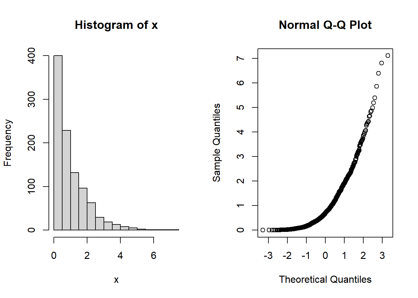
 par(mfrow=c(1,1))
 boxcox(x~1) # 로그-가능도 프로파일 생성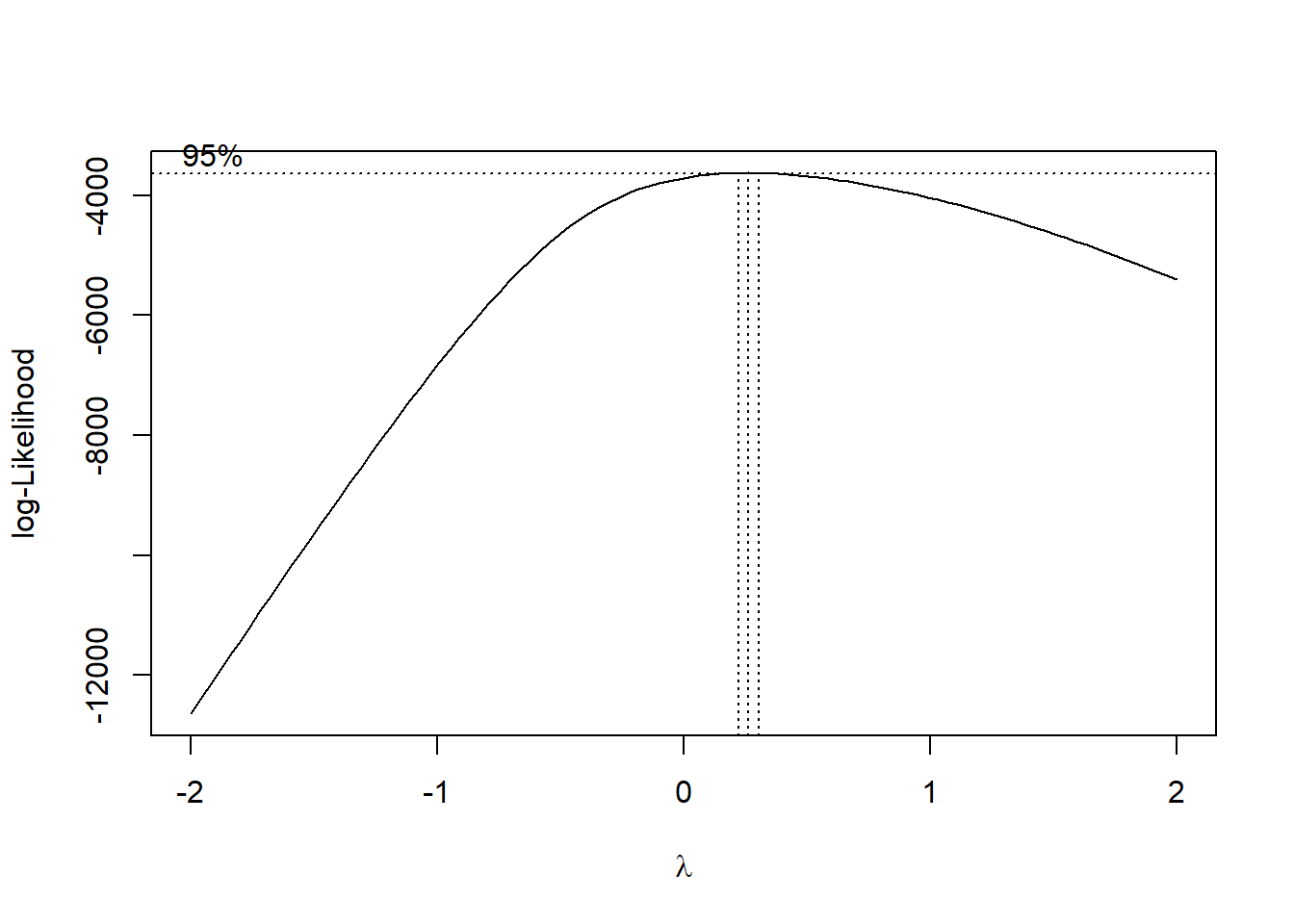
 p <- powerTransform(x) # 박스-콕스 변환의 람다 추정
p
## Estimated transformation parameter
## x
## 0.2631179 y <- bcPower(x, p$lambda) # 박스-콕스 변환
par(mfrow=c(1,2))
hist(y)
qqnorm(y) # 변환된 자료의 정규확률그림 생성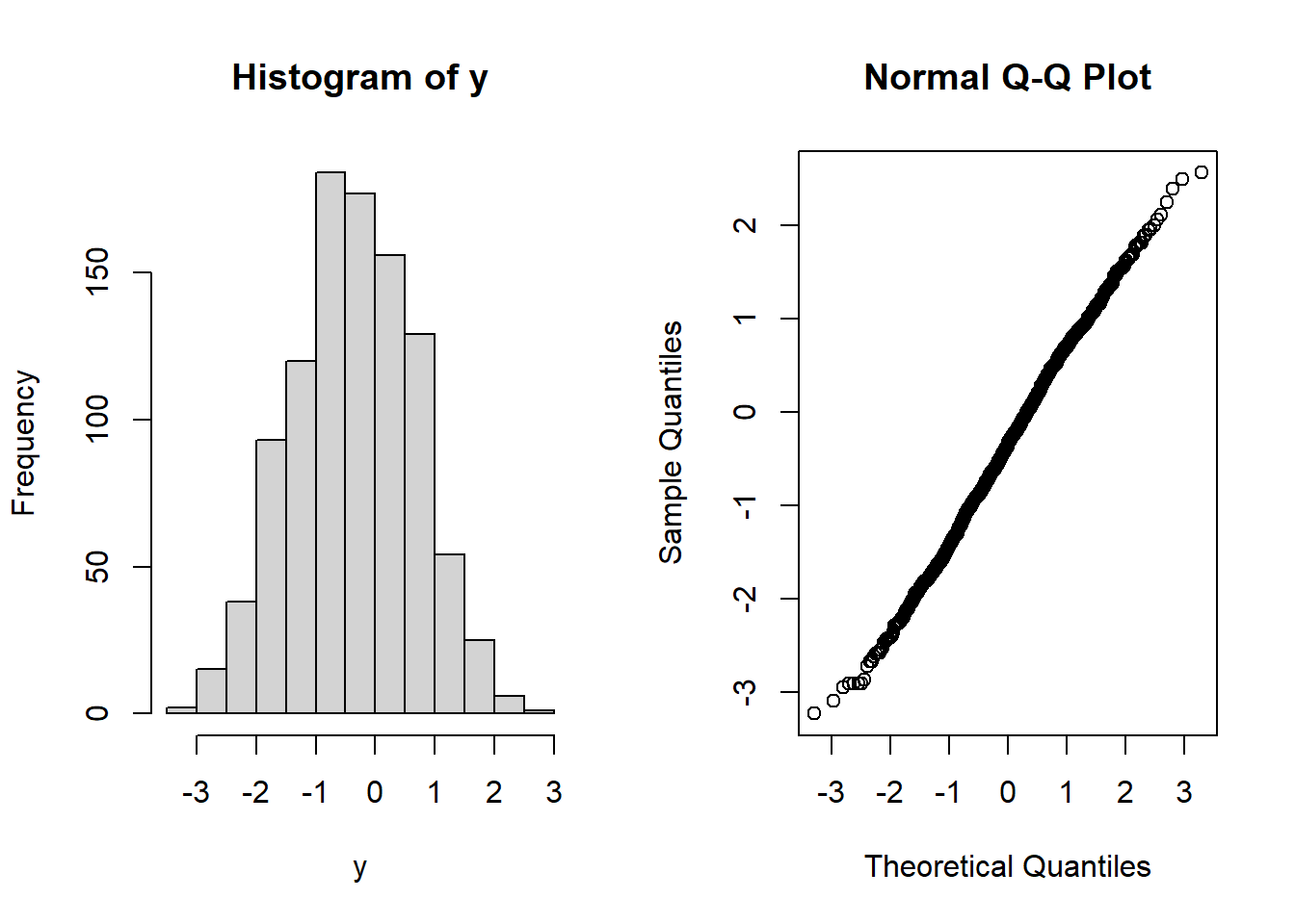
VAR모형분석
샘플을 생성한다
set.seed(111)
t <- 200 # Number of time series observations
k <- 2 # Number of endogenous variables
p <- 2 # Number of lags
상관계수 행렬 생성
A.1 <- matrix(c(-.3, .6, -.4, .5), k) # Coefficient matrix of lag 1
A.2 <- matrix(c(-.1, -.2, .1, .05), k) # Coefficient matrix of lag 2
A <- cbind(A.1, A.2) # Companion form of the coefficient matrices
예제 2
data(Canada)
summary(Canada)
## e prod rw U
## Min. :928.6 Min. :401.3 Min. :386.1 Min. : 6.700
## 1st Qu.:935.4 1st Qu.:404.8 1st Qu.:423.9 1st Qu.: 7.782
## Median :946.0 Median :406.5 Median :444.4 Median : 9.450
## Mean :944.3 Mean :407.8 Mean :440.8 Mean : 9.321
## 3rd Qu.:950.0 3rd Qu.:410.7 3rd Qu.:461.1 3rd Qu.:10.607
## Max. :961.8 Max. :418.0 Max. :470.0 Max. :12.770시도표
plot.ts(Canada) 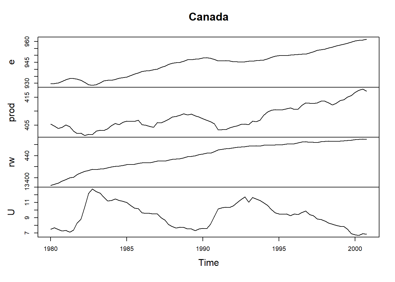 ## 단위근검정시행
adf1 <- summary(ur.df(Canada[, "prod"], type = "trend", lags = 2)) #비정상추세있음
adf1
##
## ###############################################
## # Augmented Dickey-Fuller Test Unit Root Test #
## ###############################################
##
## Test regression trend
##
##
## Call:
## lm(formula = z.diff ~ z.lag.1 + 1 + tt + z.diff.lag)
##
## Residuals:
## Min 1Q Median 3Q Max
## -2.19924 -0.38994 0.04294 0.41914 1.71660
##
## Coefficients:
## Estimate Std. Error t value Pr(>|t|)
## (Intercept) 30.415228 15.309403 1.987 0.0506 .
## z.lag.1 -0.075791 0.038134 -1.988 0.0505 .
## tt 0.013896 0.006422 2.164 0.0336 *
## z.diff.lag1 0.284866 0.114359 2.491 0.0149 *
## z.diff.lag2 0.080019 0.116090 0.689 0.4927
## ---
## Signif. codes: 0 '***' 0.001 '**' 0.01 '*' 0.05 '.' 0.1 ' ' 1
##
## Residual standard error: 0.6851 on 76 degrees of freedom
## Multiple R-squared: 0.1354, Adjusted R-squared: 0.08993
## F-statistic: 2.976 on 4 and 76 DF, p-value: 0.02438
##
##
## Value of test-statistic is: -1.9875 2.3 2.3817
##
## Critical values for test statistics:
## 1pct 5pct 10pct
## tau3 -4.04 -3.45 -3.15
## phi2 6.50 4.88 4.16
## phi3 8.73 6.49 5.47변수들이 차분 1이 필요
VARselect(Canada, lag.max = 8, type = "both") #시차 2가 가장 큰작은 값을 가짐 ## $selection
## AIC(n) HQ(n) SC(n) FPE(n)
## 3 2 1 3
##
## $criteria
## 1 2 3 4 5
## AIC(n) -6.272579064 -6.636669705 -6.771176872 -6.634609210 -6.398132246
## HQ(n) -5.978429449 -6.146420347 -6.084827770 -5.752160366 -5.319583658
## SC(n) -5.536558009 -5.409967947 -5.053794411 -4.426546046 -3.699388378
## FPE(n) 0.001889842 0.001319462 0.001166019 0.001363175 0.001782055
## 6 7 8
## AIC(n) -6.307704843 -6.070727259 -6.06159685
## HQ(n) -5.033056512 -4.599979185 -4.39474903
## SC(n) -3.118280272 -2.390621985 -1.89081087
## FPE(n) 0.002044202 0.002768551 0.00306012결과를 보면 각자 다른 차수를 추천
$selection
AIC(n)  HQ(n)  SC(n) FPE(n)
3      2      1      3
sc가 추천해준 시차 1
Canada <- Canada[, c("prod", "e", "U", "rw")]
p1ct <- VAR(Canada, p = 1, type = "both")
p1ct
##
## VAR Estimation Results:
## =======================
##
## Estimated coefficients for equation prod:
## =========================================
## Call:
## prod = prod.l1 + e.l1 + U.l1 + rw.l1 + const + trend
##
## prod.l1 e.l1 U.l1 rw.l1 const trend
## 0.96313671 0.01291155 0.21108918 -0.03909399 16.24340747 0.04613085
##
##
## Estimated coefficients for equation e:
## ======================================
## Call:
## e = prod.l1 + e.l1 + U.l1 + rw.l1 + const + trend
##
## prod.l1 e.l1 U.l1 rw.l1 const
## 0.19465028 1.23892283 0.62301475 -0.06776277 -278.76121138
## trend
## -0.04066045
##
##
## Estimated coefficients for equation U:
## ======================================
## Call:
## U = prod.l1 + e.l1 + U.l1 + rw.l1 + const + trend
##
## prod.l1 e.l1 U.l1 rw.l1 const trend
## -0.12319201 -0.24844234 0.39158002 0.06580819 259.98200967 0.03451663
##
##
## Estimated coefficients for equation rw:
## =======================================
## Call:
## rw = prod.l1 + e.l1 + U.l1 + rw.l1 + const + trend
##
## prod.l1 e.l1 U.l1 rw.l1 const trend
## -0.22308744 -0.05104397 -0.36863956 0.94890946 163.02453066 0.07142229summary(p1ct, equation = "e") #e 시계열만 보여줌##
## VAR Estimation Results:
## =========================
## Endogenous variables: prod, e, U, rw
## Deterministic variables: both
## Sample size: 83
## Log Likelihood: -207.525
## Roots of the characteristic polynomial:
## 0.9504 0.9504 0.9045 0.7513
## Call:
## VAR(y = Canada, p = 1, type = "both")
##
##
## Estimation results for equation e:
## ==================================
## e = prod.l1 + e.l1 + U.l1 + rw.l1 + const + trend
##
## Estimate Std. Error t value Pr(>|t|)
## prod.l1 0.19465 0.03612 5.389 7.49e-07 ***
## e.l1 1.23892 0.08632 14.353 < 2e-16 ***
## U.l1 0.62301 0.16927 3.681 0.000430 ***
## rw.l1 -0.06776 0.02828 -2.396 0.018991 *
## const -278.76121 75.18295 -3.708 0.000392 ***
## trend -0.04066 0.01970 -2.064 0.042378 *
## ---
## Signif. codes: 0 '***' 0.001 '**' 0.01 '*' 0.05 '.' 0.1 ' ' 1
##
##
## Residual standard error: 0.4701 on 77 degrees of freedom
## Multiple R-Squared: 0.9975, Adjusted R-squared: 0.9973
## F-statistic: 6088 on 5 and 77 DF, p-value: < 2.2e-16
##
##
##
## Covariance matrix of residuals:
## prod e U rw
## prod 0.469517 0.06767 -0.04128 0.002141
## e 0.067667 0.22096 -0.13200 -0.082793
## U -0.041280 -0.13200 0.12161 0.063738
## rw 0.002141 -0.08279 0.06374 0.593174
##
## Correlation matrix of residuals:
## prod e U rw
## prod 1.000000 0.2101 -0.1728 0.004057
## e 0.210085 1.0000 -0.8052 -0.228688
## U -0.172753 -0.8052 1.0000 0.237307
## rw 0.004057 -0.2287 0.2373 1.000000ser11 <- serial.test(p1ct, lags.pt = 16, type = "PT.asymptotic") #포트만토검정
ser11$serial##
## Portmanteau Test (asymptotic)
##
## data: Residuals of VAR object p1ct
## Chi-squared = 233.5, df = 240, p-value = 0.606var.2c <- VAR(Canada, p = 2, type = "const")
predict(var.2c, n.ahead = 8, ci = 0.95)## $prod
## fcst lower upper CI
## [1,] 417.2623 415.9835 418.5411 1.278808
## [2,] 417.7410 415.7854 419.6965 1.955532
## [3,] 418.2196 415.7674 420.6717 2.452134
## [4,] 418.5639 415.6897 421.4380 2.874136
## [5,] 418.7644 415.5065 422.0224 3.257935
## [6,] 418.8374 415.2253 422.4494 3.612043
## [7,] 418.8097 414.8748 422.7446 3.934890
## [8,] 418.7110 414.4881 422.9340 4.222973
##
## $e
## fcst lower upper CI
## [1,] 962.6557 961.9446 963.3668 0.7111044
## [2,] 963.6538 962.3422 964.9654 1.3116050
## [3,] 964.6932 962.8261 966.5603 1.8670903
## [4,] 965.6882 963.3092 968.0671 2.3789396
## [5,] 966.5814 963.7240 969.4387 2.8573301
## [6,] 967.3460 964.0344 970.6576 3.3116112
## [7,] 967.9769 964.2302 971.7236 3.7467269
## [8,] 968.4827 964.3193 972.6461 4.1633974
##
## $U
## fcst lower upper CI
## [1,] 6.428832 5.880708 6.976957 0.5481244
## [2,] 5.903919 5.017510 6.790327 0.8864083
## [3,] 5.396177 4.219319 6.573035 1.1768580
## [4,] 4.949219 3.518061 6.380377 1.4311576
## [5,] 4.595008 2.932516 6.257500 1.6624923
## [6,] 4.343933 2.463420 6.224445 1.8805126
## [7,] 4.191928 2.102592 6.281265 2.0893366
## [8,] 4.126745 1.837864 6.415625 2.2888805
##
## $rw
## fcst lower upper CI
## [1,] 470.2954 468.7660 471.8247 1.529348
## [2,] 470.8948 468.8195 472.9701 2.075289
## [3,] 471.5360 469.0592 474.0128 2.476757
## [4,] 472.2490 469.4525 475.0456 2.796577
## [5,] 473.0652 469.9976 476.1329 3.067654
## [6,] 473.9943 470.6851 477.3035 3.309184
## [7,] 475.0275 471.4966 478.5584 3.530898
## [8,] 476.1454 472.4082 479.8825 3.737164