AR(1)생성하기

x<-arima.sim(list(ma=0.2), n=100)
ts.plot(x, main="x")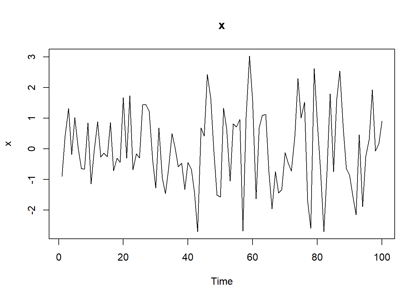

par(mfrow=c(3,1))
acf(x, main="ACF")
pacf(x, main="PACF")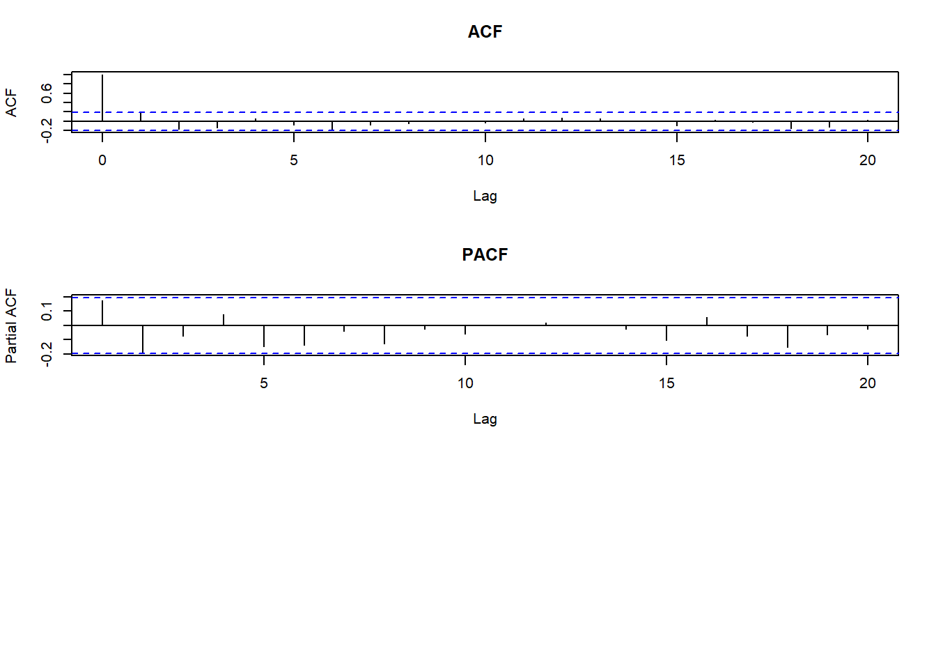

MA(1)생성하기

x<-arima.sim(list(ma=0.8), n=100)
ts.plot(x, main="x")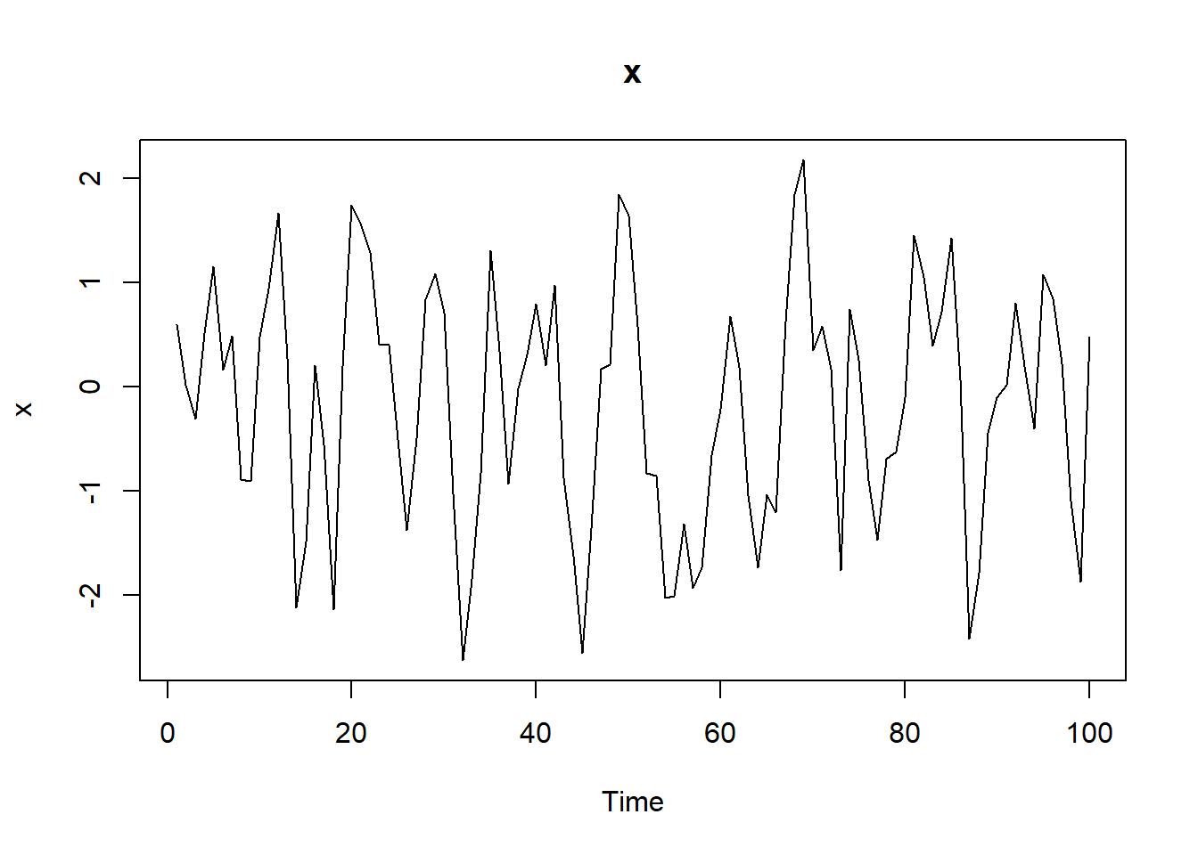

par(mfrow=c(3,1))
acf(x, main="ACF ")
pacf(x, main="PACF ")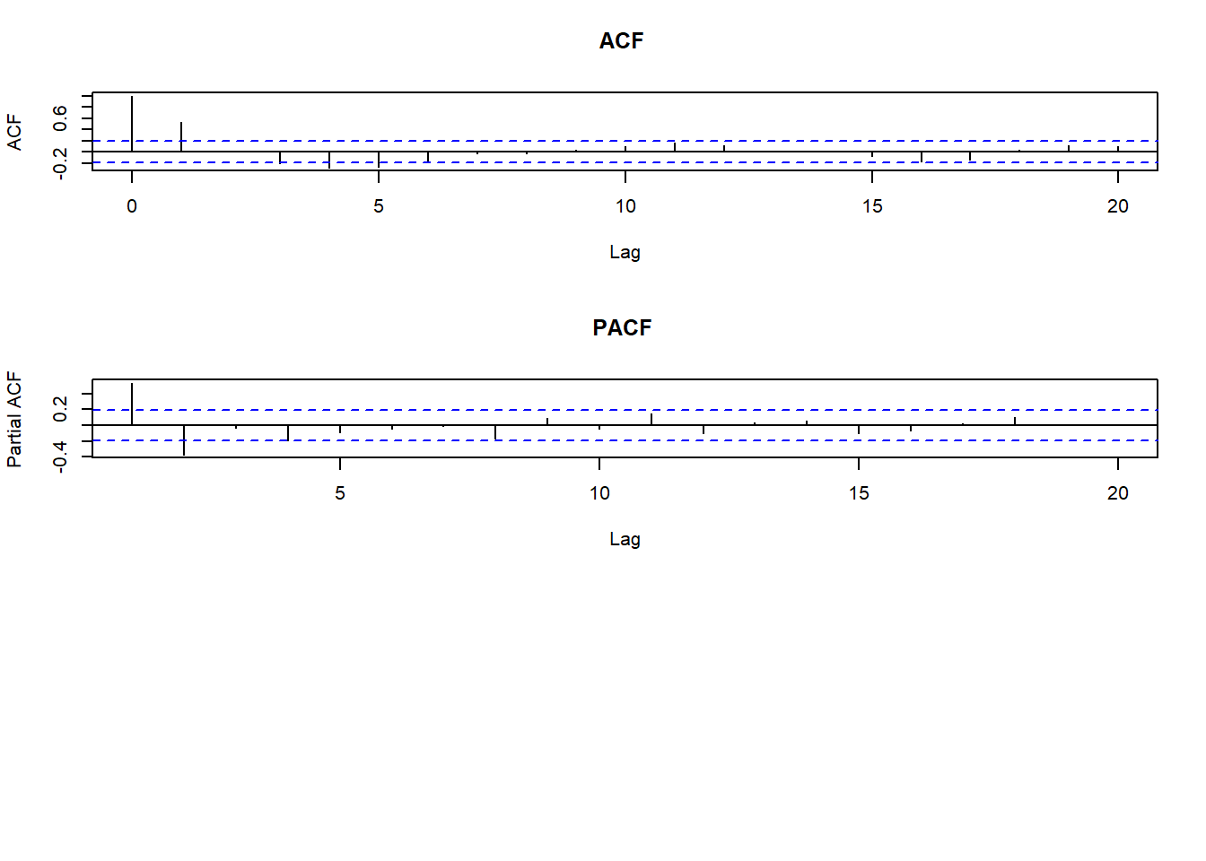

ARMA(1,1)생성하기

x<-arima.sim(list(ar=0.4, ma=-0.3), n=100)
ts.plot(x, main="x")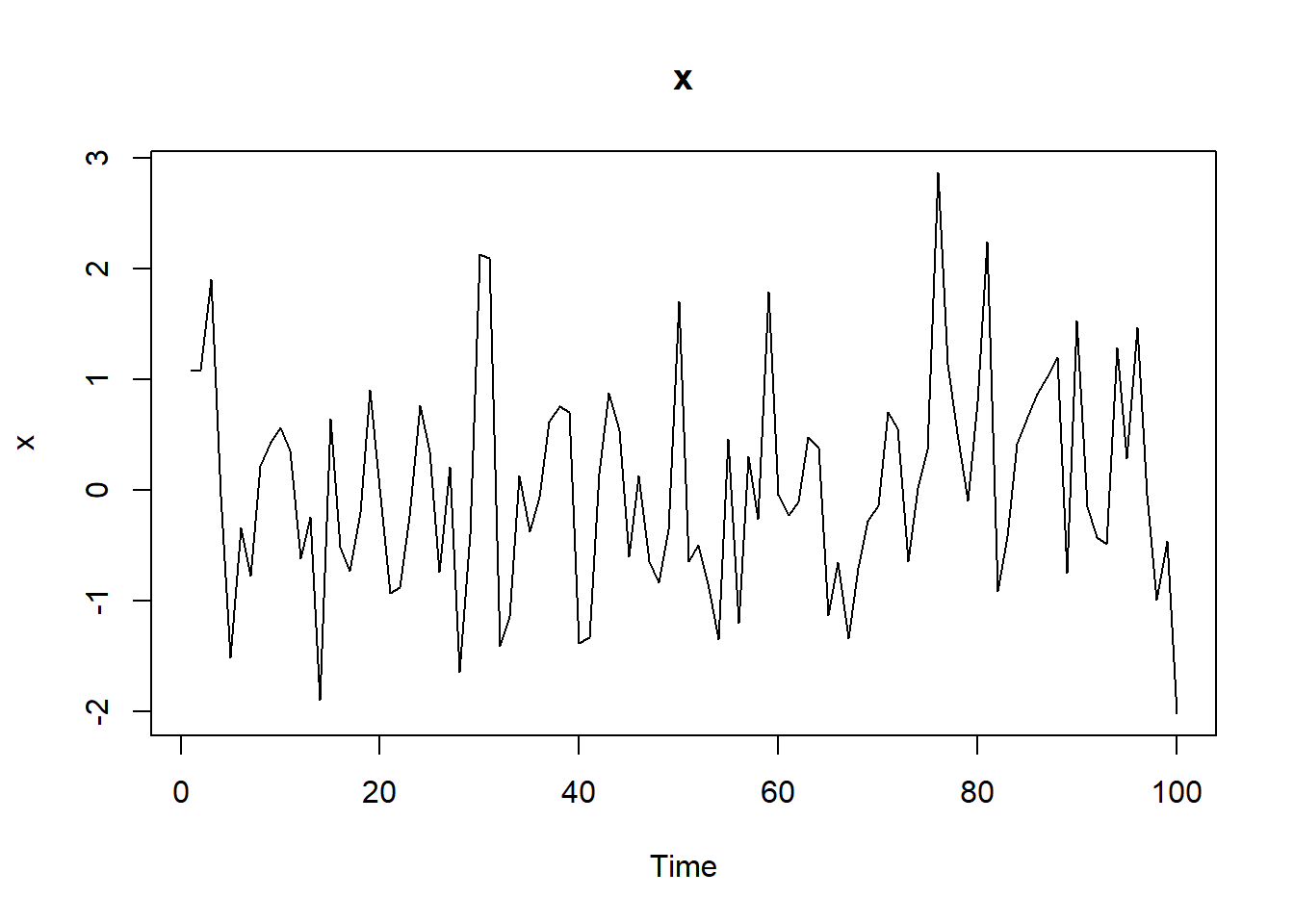

par(mfrow=c(3,1))
acf(x, main="ACF ")
pacf(x, main="PACF ") 

모형 식별하기

ts.plot(Y)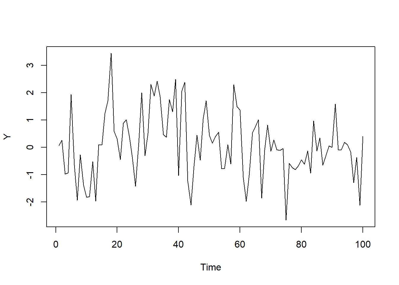

par(mfrow=c(2,1))
acf(Y, main="ACF ")
pacf(Y, main="PACF ")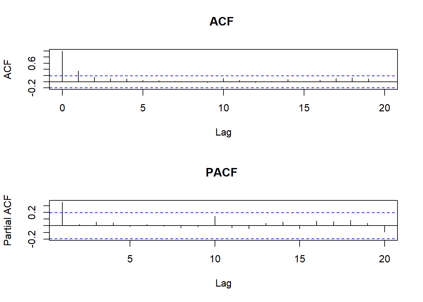

## 모수 추정해보기

TS1 <- arima(Y, c(2, 0, 0))
TS1

## 
## Call:
## arima(x = Y, order = c(2, 0, 0))
## 
## Coefficients:
##          ar1     ar2  intercept
##       0.3455  0.0208     0.0928
## s.e.  0.0999  0.1012     0.1756
## 
## sigma^2 estimated as 1.253:  log likelihood = -153.24,  aic = 314.48

TS1 <- arima(Y, c(2, 0, 0), method=c("CSS-ML"))
TS1

## 
## Call:
## arima(x = Y, order = c(2, 0, 0), method = c("CSS-ML"))
## 
## Coefficients:
##          ar1     ar2  intercept
##       0.3455  0.0208     0.0928
## s.e.  0.0999  0.1012     0.1756
## 
## sigma^2 estimated as 1.253:  log likelihood = -153.24,  aic = 314.48

TS1 <- arima(Y, c(2, 0, 0), method=c("ML"))
TS1

## 
## Call:
## arima(x = Y, order = c(2, 0, 0), method = c("ML"))
## 
## Coefficients:
##          ar1     ar2  intercept
##       0.3455  0.0208     0.0928
## s.e.  0.0999  0.1012     0.1756
## 
## sigma^2 estimated as 1.253:  log likelihood = -153.24,  aic = 314.48

TS1 <- arima(Y, c(2, 0, 0), method=c("CSS"))
TS1

## 
## Call:
## arima(x = Y, order = c(2, 0, 0), method = c("CSS"))
## 
## Coefficients:
##          ar1     ar2  intercept
##       0.3490  0.0212     0.0905
## s.e.  0.1005  0.1022     0.1795
## 
## sigma^2 estimated as 1.278:  log likelihood = -154.17,  aic = NA

모형 진단해보기

tsdiag(TS1, gof.lag=14)

## 모형 예측하기

future10<-predict(TS1, n.ahead=10)
future10

## $pred
## Time Series:
## Start = 101 
## End = 110 
## Frequency = 1 
##  [1] 0.15294742 0.11891761 0.10171254 0.09498660 0.09227444 0.09118529
##  [7] 0.09074767 0.09057185 0.09050120 0.09047282
## 
## $se
## Time Series:
## Start = 101 
## End = 110 
## Frequency = 1 
##  [1] 1.130602 1.197460 1.208324 1.210059 1.210339 1.210385 1.210392 1.210393
##  [9] 1.210393 1.210393

Upper<-future10$pred+future10$se
Lower<-future10$pred-future10$se
Upper

## Time Series:
## Start = 101 
## End = 110 
## Frequency = 1 
##  [1] 1.283549 1.316378 1.310036 1.305046 1.302614 1.301570 1.301140 1.300965
##  [9] 1.300895 1.300866

Lower

## Time Series:
## Start = 101 
## End = 110 
## Frequency = 1 
##  [1] -0.9776541 -1.0785426 -1.1066113 -1.1150728 -1.1180651 -1.1191994
##  [7] -1.1196443 -1.1198213 -1.1198922 -1.1199206

forecast(TS1,h=10)

##     Point Forecast     Lo 80    Hi 80     Lo 95    Hi 95
## 101     0.15294742 -1.295977 1.601872 -2.062991 2.368886
## 102     0.11891761 -1.415689 1.653525 -2.228061 2.465897
## 103     0.10171254 -1.446817 1.650242 -2.266559 2.469984
## 104     0.09498660 -1.455767 1.645740 -2.276686 2.466659
## 105     0.09227444 -1.458838 1.643387 -2.279947 2.464496
## 106     0.09118529 -1.459985 1.642356 -2.281125 2.463496
## 107     0.09074767 -1.460432 1.641927 -2.281577 2.463072
## 108     0.09057185 -1.460609 1.641753 -2.281755 2.462899
## 109     0.09050120 -1.460680 1.641683 -2.281826 2.462829
## 110     0.09047282 -1.460709 1.641654 -2.281855 2.462800

plot(forecast(TS1,h=10))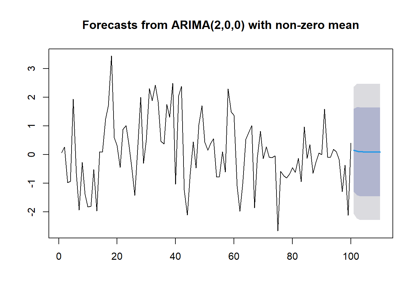

차수 식별

auto.arima(Y)

## Series: Y 
## ARIMA(1,0,0) with zero mean 
## 
## Coefficients:
##          ar1
##       0.3567
## s.e.  0.0927
## 
## sigma^2 estimated as 1.27:  log likelihood=-153.41
## AIC=310.81   AICc=310.94   BIC=316.02